In flight test as in other disciplines, measurement and calculation result in different types of errors. Some of these errors are not systematic but are random. Often we call these measurement errors noise, and it is these errors that are the focus of this section. Furthermore, it is a commonly accepted practice that the normal distribution is a suitable model for noise and measurement errors. It is imperative to emphasize that the normal distribution is just a model, a simplification of the physical world. The purpose of this next section is to demonstrate why this is a suitable model and a very relevant one.
Suppose that we are going to measure airspeed, x, with some transducer. Suppose further that at each step in the measurement process we have one of two hypothetical outcomes:
1. We measure airspeed correctly; that is, the error is zero: ε = 0.
2. Or there is some error in our measurement of airspeed, which we model as follows: ε = 1.
In other words, we have a model that returns 0 when there is no error and 1 when there is.
| Measurement process | After a single step or factor in measurement process:x + ε |
| Possible outcomes | x x + 1 |
Suppose that there are two steps that affect the given measurement. For example, measurement of airspeed requires both static and dynamic pressure. The error term propagates at each step. So we have the following:
| Measurement process | After a single step or factor: x + ε | After a second step or factor: x + ε |
| Possible outcomes | x | x |
| x + 1 | ||
| x + 1 | x + 1 | |
| x + 2 |
After two steps, we can any of three possible outcomes, x, x + 1, or x + 2. But the middle outcome occurred twice. Imploring upon your patience, consider outcomes after three steps.
| Measurement process | After a single step:x + ε | After second step:x + ε | After third step:x + ε |
| Possible outcomes | x | x | x |
| x + 1 | |||
| x + 1 | x + 1 | ||
| x + 2 | |||
| x + 1 | x + 1 | x + 1 | |
| x + 2 | |||
| x + 2 | x + 2 | ||
| x + 3 |
Another way to see how these tables propagate is in the tree of figure 1. At each node of the tree, the value in the node represents the cumulative error, and the two branches indicate that there are two possible outcomes either +0 or +1.

Thus after three steps or factors in the measurement process, there are four possible unique outcomes, x, x+1, x+2, x+3, but two of these outcomes occur more than once. In other words, there is more than one possible path through the tree to certain nodes. We can record the different outcomes and the frequency with which they occur in a rudimentary table as follows:
| Number of occurrences | I | I I I | I I I | I |
| Outcome, x+ ε | x + 0 | x + 1 | x + 2 | x + 3 |
This table allows us to picture qualitatively, based on the height of the tallies, the relative frequency of each particular outcome. It also allows us to quantitatively compute the probabilities of a given outcome. Thus, P(x+0) is the probability of no error in the measurement, and it is a ratio given by (number of times given outcome occurs) / (number of total possible outcomes) = 1 / 8; in other words, the number of tallies in a given column / total number of tallies.
The reader may continue this exercise for several more iterations and see two important principles:
1. Simple probabilities like the toss of a coin (a fifty-fifty chance) can quickly compound and propagate into more complex distributions.
2. There is a formula with which we can compute the number of occurrences in this discrete model, the binomial distribution.
Definition: Binomial Distribution
The binomial distribution is the probability of obtaining exactly n outcomes in N trials.
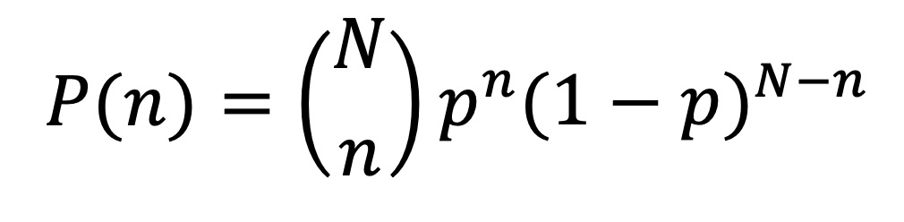
From our example worked thus far, we could compute the probability of obtaining n errors in N stages or factors of the measurement process, that is, P(obtaining x + ε as the outcome) for ε=0, 1, 2, or 3. In this case N = 3 when we examine the outcome after 3 stages or factors in our measurement process.
| Number of occurrences | l | lll | lll | l |
| Outcome, x+ ε | x + 0 | x + 1 | x + 2 | x + 3 |
| P(x + ε) | P(ε=0)=1/8 | P(ε=1)=3/8 | P(ε=2)=3/8 | P(ε=3)=1/8 |
We let n = 0, 1, 2, or 3, based on whether we want to know the probability of the outcome x+0, x+1, x+2, or x+3, respectively. Additionally, p is the probability of the error at each stage. For the purpose of our example, we can say that ε = 0 or 1 are equally likely, and thus we assign p = 1/2. Microsoft Excel or Google spreadsheets, MATLAB or python, and many other tools have functions that allow us to compute these probabilities.
Modeling Error with the Normal Distribution
Up to this point, our example has highlighted use of the binomial distribution, a model capable of handling discrete cases. In other words, we can compute the probability for any N = 1, 2, 3… including any whole number value. However, this model cannot accept continuous values, and it is cumbersome for even nominally large values of N—it becomes an unnecessary burden on memory and computational resources. There is a natural relationship between the binomial distribution and the normal distribution, and the bell curve is an excellent model for continuous and fractional measurement errors.
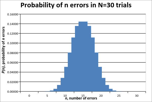
Consider the bar chart of probabilities of the binomial distribution with N = 30 and p = ½. The chart shows us all the possible values of P(n), the probability of n errors in N = 30 trials. For example, if we compute P(n=15) using the formula for the binomial distribution, we would find that P(15) = 0.14446. We also see that the height of the bar at n=15 is 0.14446. The x-axis depicts n, and we can see that it ranges from 0 to 30, and the y-axis is the probability P(n), a number between 0 and 1. Recall that in our example of propagating errors, we were counting the number of errors (ε) after a certain number of steps or factors. Thus n is equivalent to the number of errors, and N is equivalent to the number of steps or factors. As we can see, the shape of this discrete distribution begins to resemble the familiar bell curve shape of the normal distribution.
Consider now a continuous model of measurement error. Suppose again that we are going to measure airspeed, x, with some transducer. Suppose further that at each step in the measurement process we can have fractional errors. In other words, we measure 202.5 when the truth is x = 200 knots. Here we have as the error term ε = 2.5, as an example. This is more like the physical reality than the binomial example above. To describe it adequately, we need the following additional definition.
Definition: Normal Distribution
The bell curve is formally known as the normal distribution and is the continuous probability distribution given by the probability density function below, where µ, the mean, and σ, standard deviation, are given.
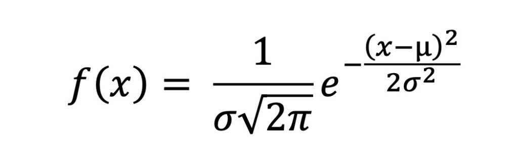
Practically speaking, the parameters µ and σ, help us define the shape of the bell curve, whether it is tall and skinny or short and fat, for example. There are two ways to observe our measurement error. We could plot a bell curve centered at 200 knots, the truth value, or we could subtract our measured value from the truth value and obtain an error term, ε = 202.5 – 200 = 2.5. In this second case, our curve would be centered at 0.
When we plot flight test data, we normally plot the raw values, so the former may occur more naturally. Additionally, plotting error terms is not always analytically tractable, and thus it is advantageous to plot the raw data. However, strictly speaking, it is the error term that we model with a normal distribution, not the airspeed term. Therefore, one must apply great care to avoid the mistakes in reason caused by a misunderstanding of what data are actually normally distributed.
Conclusion
This has been a very quick introduction to noise and the normal distribution, a vital tool that we use to model noise in flight test data, and we will close with one example that uses this tool: RNAV and RNP.
Flight test is the place where validation of the accuracy of navigation systems occurs by comparison to a truth position source, and understanding the normal distribution is essential to applying the definitions of RNAV and RNP.
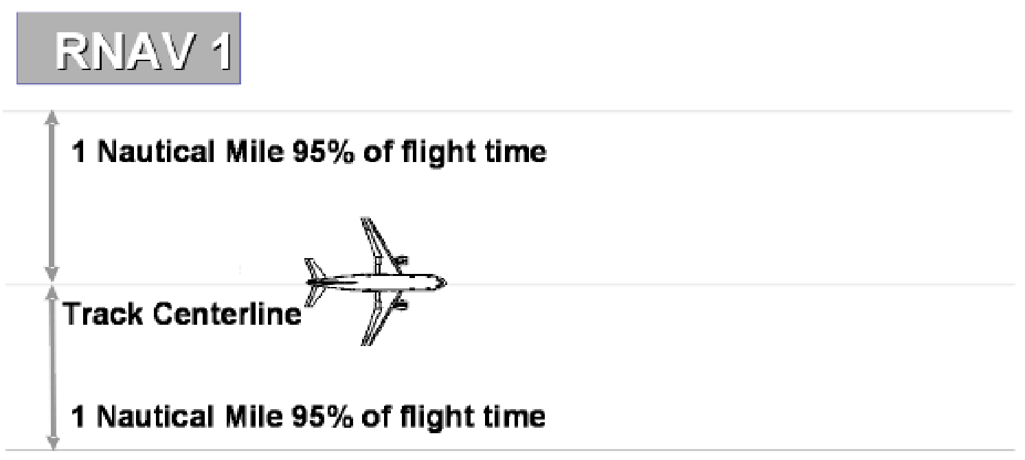
Figure 1 is from an FAA advisory circular and illustrates the definition of RNAV. Ninety-five percent is a common value used in many confidence intervals, based on approximately two standard deviations from the mean, and it is this concept used in the definition of RNAV. We won’t take the time to discuss the subtleties of confidence intervals here, however.
In this second illustration, also from an FAA advisory circular, we see the definition of RNP. Again, confidence intervals are brought to bear on the navigation position, but this time, we see a much higher level of confidence, one exceeding three standard deviations from the mean.

This article first appeared in the November 2014 Flight Test News.
One thought on “Introduction to Measurement Error”
Comments are closed.