by Al Lawless and Mark Jones Jr.
Orbis is a pitot-static Flight Test Technique especially useful in RVSM airspace that results in a highly accurate measurement of winds aloft (±0.3kts). But why should you care, and why do we discuss it here?
Since October, every other issue of FTN has featured a column with technical content, a practice we hope to continue for several reasons. First, it gives us a chance to direct the reader to the host of technical papers on our website and to highlight papers of particular relevance. We do this with the hope that you will get value from these papers and that you will appreciate the investment of time and energy from other members who wrote these papers. If, as a byproduct, it inspires you to do the hard work of writing and presenting a technical paper at a future symposium, then that is also a benefit. Second, we hope to constantly highlight our hallmark resource, the SFTE Technical Reference Handbook. In this month’s feature, we gloss over elementary pitot-static theory in hopes that you will open the Handbook and dig into the pitot-static fundamentals. Finally, and perhaps most importantly, we hope that this feature is more than just a rerun. We don’t want FTN to repeat news that was available elsewhere. Instead, we believe it can be a laboratory, a place where we introduce ideas that may not be ready for entry into service but will certainly benefit from the rigorous discussion, questioning, and counter-arguments that we expect and hope will blossom following their explanation here. That brings us full circle to Orbis.
After more than a century of flight, air data calibration is still a keystone of the flight test profession. A quick and informal survey of the SFTE technical paper database shows that pitot-statics is a frequent subject of symposia presentations, and a cursory glance at the website of the European Chapter shows a similar trend. Many of these papers introduce ideas that improve upon but do not significantly alter elementary flight test techniques (FTTs). The maturity of GPS-integrated avionics systems and improvements in applied tools of math and stats have opened a rich area of study for a new kind of air-data calibration FTT. For example, this paper suggests that GPS altitude, when correlated to trailing cone data during a constant airspeed calibration run, is a highly accurate truth source for subsequent runs using a level-acceleration FTT for air data calibration—accurate data across the operational (airspeed) envelope in fewer high altitude missions. Trailing cones are usually subject to lag errors in such a maneuver. I also mention this paper because of the potential synergy with the Orbis method.
The point of this discussion is not to explore all such GPS methods, but it will focus on one promising method that has not yet reached publication. Orbis Matching is an FTT developed by Al Lawless. He first presented these slides at a symposium in Germany, and it has been used informally in industry and academia for several years now.

The Orbis FTT is a circular, constant altitude and constant airspeed turn, flown to gather pitot-static and GPS data for comparison and calibration. Its primary advantage is a highly accurate measurement of winds aloft, especially in RVSM airspace where this accuracy is more important from a regulatory standpoint and other FTTs are not as efficient (or impossible—there is no tower-fly by FTT up there yet). The output of the Orbis FTT includes a circular scatter plot of GPS-derived groundspeed data: East component of groundspeed is on the x-axis, and North component is on the y-axis. We call this circular plot the Orbis, a Latin word that means circle.

There are, however, several important things to note about the plot. First, the plot is in fact a circle, with the exception of noise, in the sense that it is perfectly round. It is not an ellipsoid. Second, we want to emphasize an important point—the plot is not a representation of the ground track of the aircraft. Instead it is a plot of ground speed coordinate pairs, where (x, y) are the Easterly component (x) and the Northerly component (y) of groundspeed, respectively. This is another reason for referring to this plot as the Orbis, to remove the notion of ground track from our intuition. To see this more clearly, note the x and y are the ground speed at these points—if this were a representation of ground track, these intercepts would have a magnitude equal to the turn radius. Instead, they intercept at a number that looks a lot like true airspeed (200-300 knots in the above plot). Finally, note that we do not interpret this plot in the traditional sense: Here y is not a dependent variable, is not a function of x. In fact, both variables are independent in some sense, and in another sense they are both functions of some other unnamed variable(s). The point in all these is to lay aside intuition and accept the data plot as an Orbis, along with all the implicit meaning the name suggests.
From this plot, an accurate derivation of the winds aloft is possible, and together with groundspeed and ship system airspeed data, derivation of Ps follows. In the plot presented here, one can see that the center of the Orbis is offset from the origin. The wind vector corresponds to this offset, and derivation is simple.
The steady turn is one advantage of the Orbis. Existing GPS methods may use momentary stabilized headings, but these do not allow for precise wind speed determination in the real atmosphere. Better wind estimation comes at the cost of more time on condition at more headings. Addition of more straight runs (or multiple horseshoes, windboxes, cloverleafs, etc.) becomes a time consuming process and reduces the benefit of GPS methods. Orbis addresses all of these limitations by sampling at hundreds of headings without stabilization and accomplishing the sample in the short time required to fly a complete circle. An additional benefit is that higher bank angles (higher AOA) are an easy method to simulate higher weight test points. A turn is also a manevuer more suitable for RVSM airspace testing. It results in less interference than traditional methods when testing takes place in this traffic-dense, shared airspace.
One obvious concern immediately comes to mind. What if the maneuver is not flown perfectly? What about a gust of wind? What effect does this have on the air data calibration, and how might we address these limitations? These are realistic questions, and one such example of noisy data (blue) appears in Figure 1. We have added to the plot the (red) trace of uncalibrated true airspeed, as seen in Figure 1. (We call it uncalibrated true airspeed because this is pitot-static, not yet corrected, true airspeed data, denoted VT_i. The red curve is the data from the pitot-static system that we are in the process of calibrating with this FTT.)
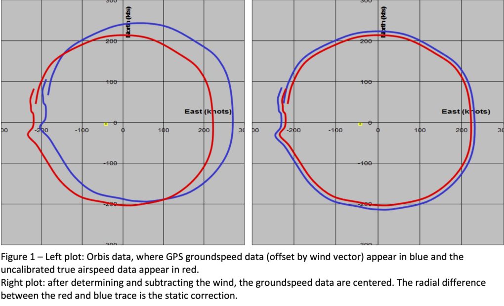
What may not be immediately intuitive, but what is apparent in the figure, is that the magnitude of anomalies in groundspeed—regardless of their cause—correlate with anomalies in true airspeed. We also point out that the true airspeed trace,VT_i. in red, is centered at the origin, because wind has no effect on it. Now by estimating the wind vector and subtracting it from the ground speed data, we may re-center the ground speed data about the origin, shown in the right half of Figure 1. Deriving the wind vector is an iterative process that begins with a rough estimate, VW, and taking the difference between the two plots: [(VGS + VW) – VT_i ]. We show this in the upper plot below. Here the airspeed difference is the y-axis, and GPS ground track is on the x-axis. The engineer repeats these steps until the curve is at flat as possible, as seen in the lower portion of Figure 2. Here, standard deviation is our quantitative measure of flatness.
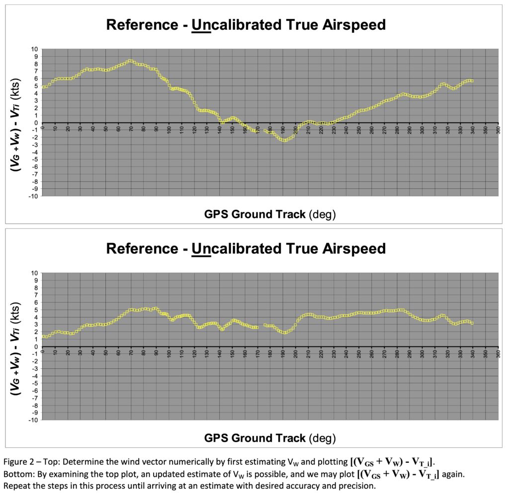
With this highly accurate wind calculation, we have finally arrived at the punchline. The bias that appears in the bottom of Figure 2 is the radial difference between the red and blue Orbis plots, and it reflects the pitot-static error. We leave the derivation to the reader. (I’ve always wanted to say that. In all seriousness, the Orbis Matching presentation presents the derivation in greater detail.)
Development and evaluation of the Orbis FTT continues following two parallel approaches. The first is actual implementation of the FTT simultaneously with traditional trailing cone methods, and this ongoing effort is the source of the data and analysis above. The second approach is a development of the mathematical model and statistical simulation in an attempt to understand Orbis from first principles. The work from this approach is also available as downloadable attachments in the SFTE forum. From this, we hope shed some light on the quantitative, numeric, and computational advantages and limitations of the Orbis. For example, we aim to answer important questions like, “how much of the orbis must be flown—what is the minimal arc in degrees—from which pitot static data may be derived with high fidelity?” This is just one of many conclusions to which development of the Orbis mathematical model may lead, together with a deeper understanding of analytical tools of mathematics and statistics. Finally, we hope to use both of these approaches to achieve synergies, e.g., harmonizing the GPS altitude approach (that Young, Jorris, Erb, et al. present in their paper) with the Orbis approach and other methods or improvements that this discussion may cultivate.
This article first appeared in the February 2015 Flight Test News.